Daniel Ciocîrlan
5 min read •

Share on:
This article is for the Scala & Spark programmers, particularly those Spark programmers that are starting to dive a little deeper into how Spark works and perhaps attempting to make it faster.
In this article, I’m going to discuss the commonalities and the differences between repartition and coalesce.
I’m going to work in an IntelliJ project with the Spark library installed, so add the following to your build.sbt file:
libraryDependencies += "org.apache.spark" %% "spark-core" % "3.0.0"
I’m also going to work in a standalone application, for which I’m going to spin up a dedicated Spark Session:
object RepartitionCoalesce {

  val spark = SparkSession.builder()
    .appName("Repartition and Coalesce")
    .master("local[*]")
    .getOrCreate()

  val sc = spark.sparkContext
}
You’re probably aware of what this code does - the SparkSession is the entry point for the high-level DataFrame API, and the SparkContext is the entry point for the low-level RDD API.
The techniques I’m going to show in this article are 100% applicable to both RDDs and DataFrames, but to demonstrate their differences, I’m going to generate more data more quickly with the RDD API.
val numbers = sc.parallelize(1 to 10000000)
println(numbers.partitions.length)
When you run this application, provided that you configured the SparkSession with local[*] master (like in the snippet), you’ll most likely see the number of your virtual cores. By default, this is how an RDD will be split. This demo will be most visible if you have more than 2 virtual cores on your computer.
Repartition is a method which is available for both RDDs and DataFrames. It allows you to change the number of partitions they are split into. This is particularly useful when your partitions are very small and data processing is slow because of it - you can hit repartition with a smaller number of partitions, and your data will be redistributed in between them. Try to repartition your data into fewer partitions than the number of cores:
val repartitionedNumbers = numbers.repartition(2)
repartitionedNumbers.count()
A repartition will incur a shuffle - a data exchange between executors in the cluster. When we deal with Spark performance, we generally want to avoid shuffles, but if it’s for a good cause, it might be worth it. Regardless of whether it’s worth it or not, repartition involves a shuffle - this is the important bit.
Another method for changing the number of partitions of an RDD or DataFrame is coalesce. It has a very similar API - just pass a number of desired partitions:
val coalescedNumbers = numbers.coalesce(2)
coalescedNumbers.count()
Let’s run a small test - execute this application with the count action executed on the two RDDs repartitioned and coalesced to 2 partitions, respectively. If you need to, add a sleep in the main thread so you can watch the Spark UI. It’ll take no more than a few seconds to run. Since we have two count actions there, we’ll have two jobs running.
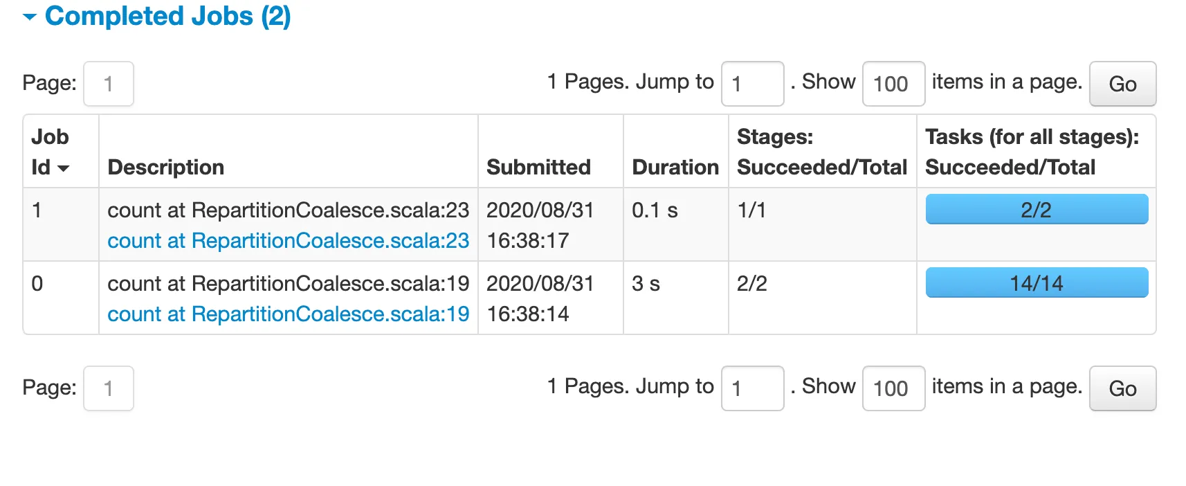
If you look at the Spark UI, you’ll see something very interesting:

The first job (repartition) took 3 seconds, whereas the second job (coalesce) took 0.1 seconds! Our data contains 10 million records, so it’s significant enough.
There must be something fundamentally different between repartition and coalesce.
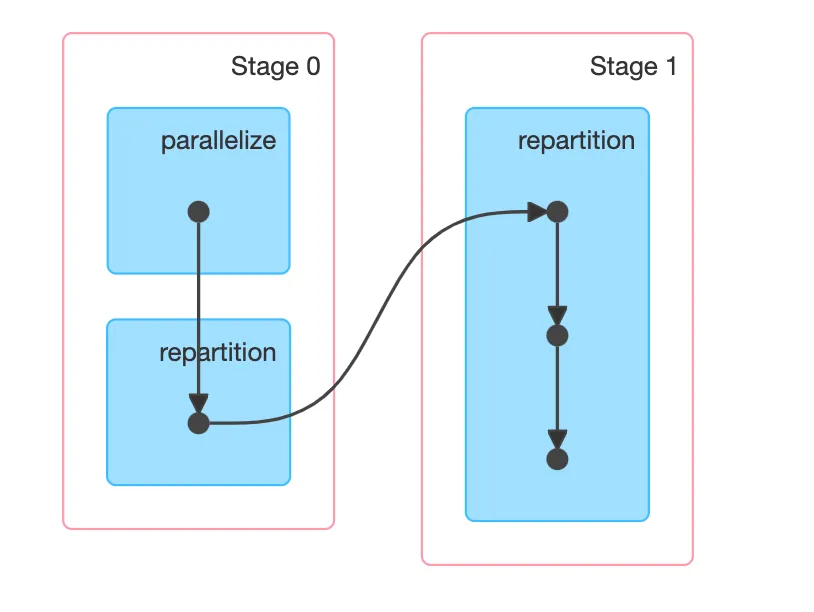
We can explain what’s happening if we look at the stage/task decomposition of both jobs. In this case, the DAGs are very useful. Let’s look at repartition:

In other words, we have two stages and a shuffle in between them. As I mentioned earlier, this is expected - a repartition will redistribute the data evenly between the new number of partitions, so a shuffle is involved. As you probably know, shuffles are expensive, even for the ~70MB of data we’re dealing with.
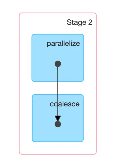
Let’s look at the other DAG of the coalesce job:

In other words, a single stage! Coalesce does not involve a shuffle. Why doesn’t it incur a shuffle since it changes the number of partitions?
Coalesce changes the number of partitions in a fundamentally different way. Instead of redistributing the data evenly between the new number of partitions, coalesce will simply “stitch” partitions together, so there’s no data movement between all executors, but only between those involved in the respective partitions.
Put in a different way: in the case of a repartition, each input partition will spread data into all output partitions. In the case of coalesce, each input partition is included in exactly one output partition. This causes massive performance improvements in the case of coalesce, when you’re decreasing the number of partitions. If you’re increasing the number of partitions, a coalesce is identical to a repartition.
So why ever do a repartition at all?
The fundamental benefit of a repartition is uniform data distribution, which a coalesce can’t guarantee - since it stitches partitions together, the output partitions might be of uneven size, which may or may not cause problems later, depending on how skewed they are.
And with that, massive performance benefits await if you know how to make the right tradeoffs, as with anything in life.
Share on: