Understanding Spark DAGs (Directed Acyclic Graphs)

Who This Article Is For

This article is for the Spark programmer who has at least some fundamentals, e.g. how to create a DataFrame and how to do basic operations like selects and joins, but has not dived into how Spark works yet. Perhaps you’re interested in boosting the performance out of your Spark jobs.

Introduction

You’re surely aware that Spark has this lazy execution model, i.e. that you write transformations but they’re not actually run until you call an action, like a show, or collect, or take, etc.

When you write transformations, Spark will automatically build up a dependency graph of your DataFrames, which will actually end up executing when you call an action.

val simpleNumbers = spark.range(1, 1000000)
val times5 = simpleNumbers.selectExpr("id * 5 as id")

That times5 DataFrame will not actually get evaluated until you call an action, like

times5.show()

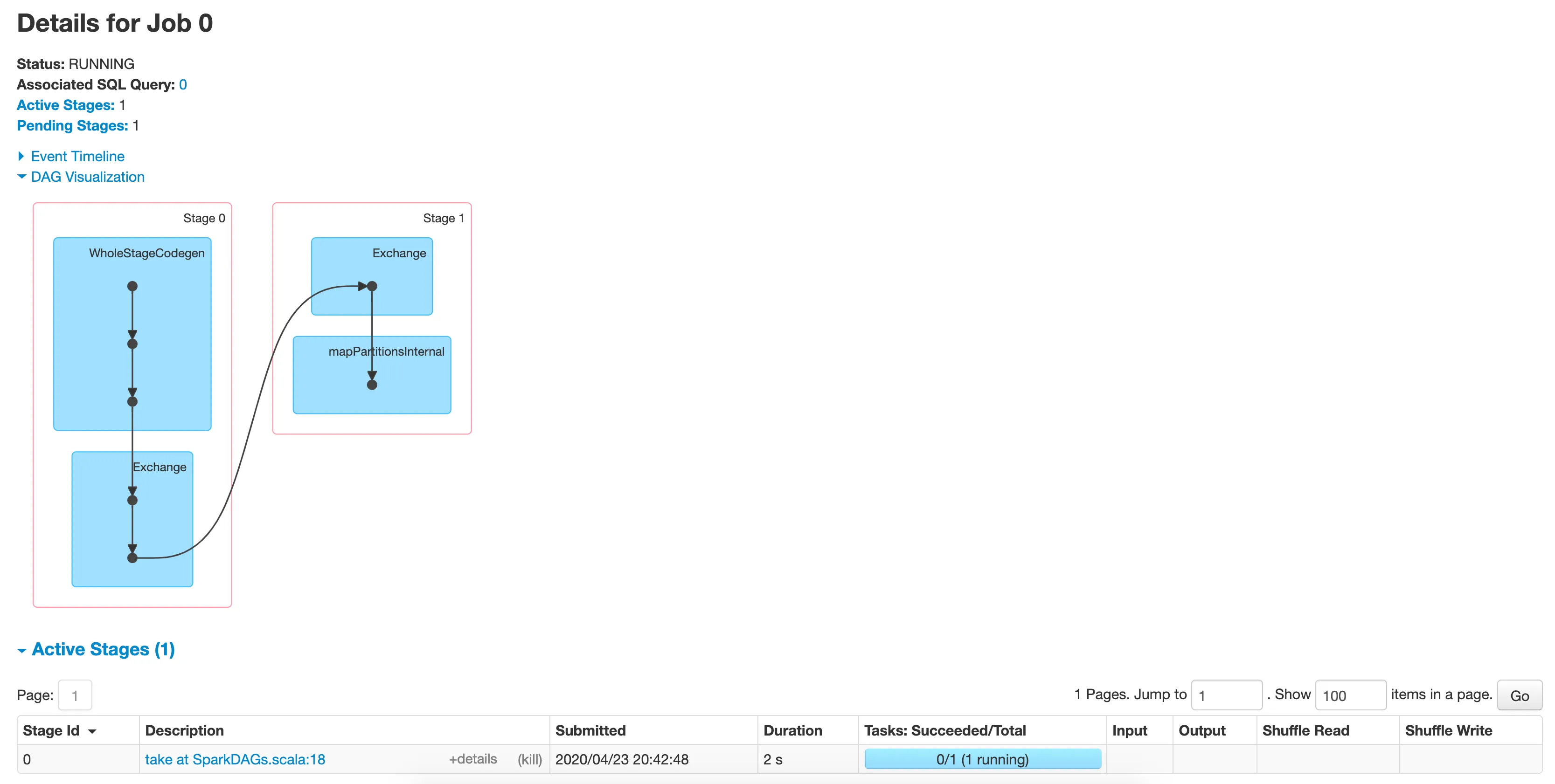
Only at this point will Spark be performing the actual computations. An action will trigger a Spark job, which will be visible in the Spark UI. If you run this locally, either in your IDE or on your Spark Shell, usually the Spark UI will be at localhost:4040. When you go to the Spark UI, you’ll see a table with all the jobs that the application has completed and is currently running. If you click on the one you just ran, you’ll see something like this:

The cute diagram with the blue boxes is called the Directed Acyclic Graph, or DAG for short. This is a visual description of all the steps Spark will need to perform in order to complete your computation. This particular DAG has two steps: one that is called WholeStageCodegen, which is what happens when you run computations on DataFrames and generates Java code to build underlying RDDs - the fundamental distributed data structures Spark natively understands - and a mapPartitions, which runs a serial computation over each of the RDD’s partitions - in our case multiplying each element by 5.

Every job will have a DAG, and usually they’re more complicated than this.

Prerequisites

The code I’ll be writing is inside a Spark shell with version 3.0.0, which you can find here for download. The default choices in the dropdown selectors will give you a pre-compiled Spark distribution. Just download, unzip, navigate to the bin folder, then run the spark-shell executable.

That is, if you’ve never installed Spark before.

Understanding DAGs

So let’s go over some examples of query plans and how to read them.

val moreNumbers = spark.range(1, 10000000, 2)
val split7 = moreNumbers.repartition(7)
split7.take(2)

Same operation first, but the next step is an Exchange, which is another name for a shuffle. You’re probably aware - a shuffle is an operation in which data is exchanged (hence the name) between all the executors in the cluster. The more massive your data and your cluster is, the more expensive this shuffle will be, because sending data over takes time. For performance reasons, it’s best to keep shuffles to a minimum.

Also notice that after this shuffle, the next steps of the DAG are on another “column”, it’s like another vertical sequence started. This is a stage. After every Exchange will follow another stage. Exchanges (aka shuffles) are the operations tha happen in between stages. This is how Spark decomposes a job into stages.

Let’s do one more, this time make it complex:

val ds1 = spark.range(1, 10000000)
val ds2 = spark.range(1, 10000000, 2)
val ds3 = ds1.repartition(7)
val ds4 = ds2.repartition(9)
val ds5 = ds3.selectExpr("id * 5 as id")
val joined = ds5.join(ds4, "id")
val sum = joined.selectExpr("sum(id)")
sum.show()

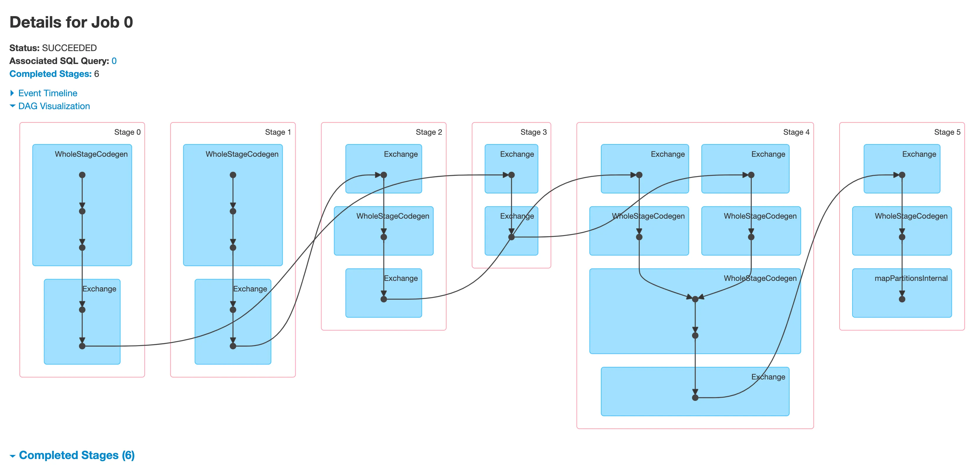
Now that’s a nasty one. Let’s take a look.

A good intuitive way to read DAGs is to go up to down, left to right. So in our case we have the following.

We start with Stage 0 with a familiar WholeStageCodegen and an exchange, which corresponds to the first DataFrame which gets repartitioned into 7 partitions. A very similar thing for stage 1. These two stages are not dependent on one another and can be run in parallel.

In Stage 2, we have the end part of the Exchange and then another Exchange! This corresponds to ds4, which has just been repartitioned and is prepared for a join in the DataFrame we called “joined” in the code above. You probably know that Spark usually performs a shuffle in order to run a join correctly. That is because the rows with the same key need to be on the same executor, so the DataFrames need to be shufffled.

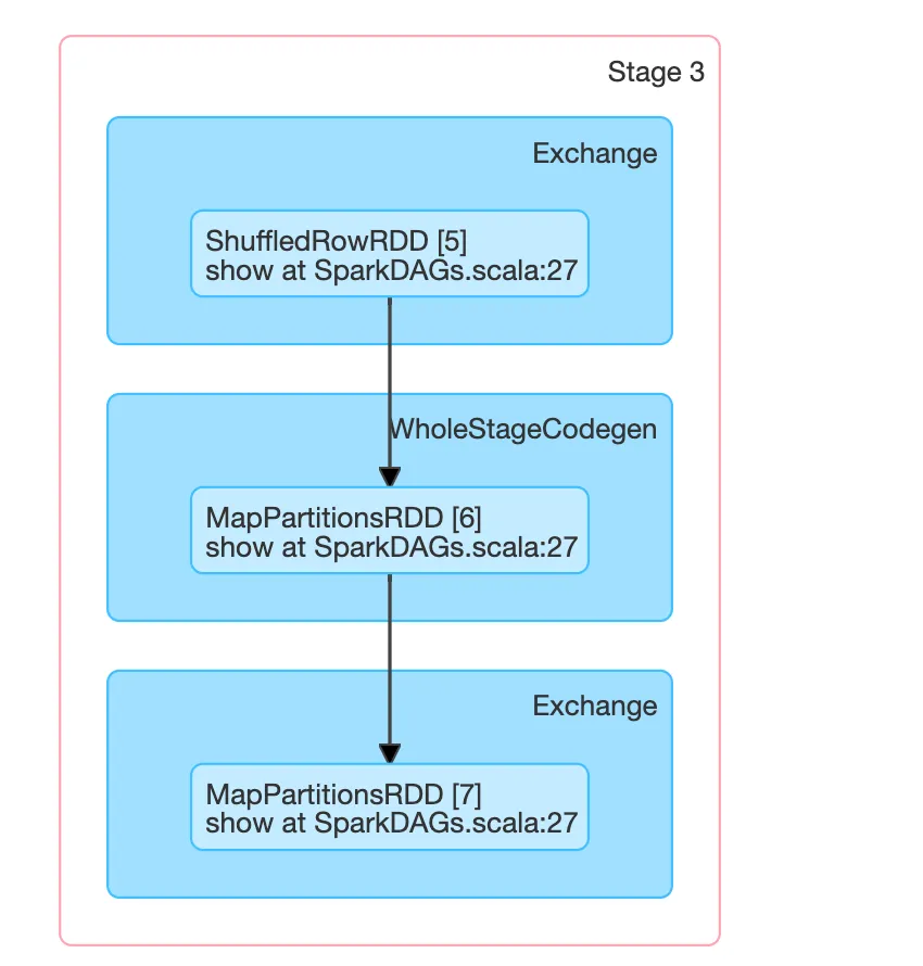
In Stage 3, we have a similar structure, but with a WholeStageCodegen in between. If you click on this stage, you’ll see what this actually means:

In the box where it says WholeStageCodegen, you’ll actually see the RDD implementation that Spark will use. In our case, that’s a MapPartitionsRDD, which simply means that a serial operation was run on the entries in each partition of this RDD, in parallel. This corresponds to the DataFrame we called ds5 in the code, because multiplying each element by 5 can be done individually on each record, in parallel. So another lesson here: this kind of select statements - where you don’t do any aggregations - are highly parallelizable and good for performance.

Next, in Stage 4, we have the big join operation. You probably spotted it right in the middle. Before it does the join, Spark will prepare the RDDs to make sure that the records with the same key are on the same executor, which is why you’re seeing some intermediate steps before that. At the end of Stage 4, we have - you guessed it - another shuffle.

That’s because in Stage 5, Spark will need to bring all the data to a single executor in order to perform the final computation, because we’re doing a massive aggregation on the entire DataFrame. So another lesson here: aggregations usually involve some form of moving data between executors, which means a shuffle. “Group by” statements are particularly sensitive here. Because shuffle is bad for perf, then it follows that groups and aggregations can be bad for perf, so use them sparingly.

Conclusion: This Is Just the Beginning

This seems tedious, but in practice, the skill of reading and interpreting DAGs is invaluable for performance analysis. You might notice that in the last example, we’re doing quite a few shuffles. With time, you will learn to quickly identify which transformations in your code are going to cause a lot of shuffling and thus performance issues.